逻辑回归是一个应用于监督学习、用于解决二分类(0 or 1)问题的机器学习算法,用于估计某种事物的可能性,其目的是最小化预测值与真实值的误差。
逻辑回归算法评估概率:𝐺𝑖𝑣𝑒𝑛 𝑥, 𝑦̂=𝑃(𝑦=1|𝑥), where 0≤𝑦̂≤1。
参数设置
输入的特征向量:𝑥 ∈ R𝑛𝑥,𝑛𝑥是特征数量
标签:𝑦 ∈ 0,1
权值:𝑤 ∈ R𝑛𝑥, 𝑛𝑥是特征数量
阈值:𝑏 ∈ R
输出:𝑦̂ = 𝜎(𝑤𝑇𝑥 + 𝑏)
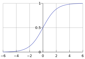
Sigmoid函数:s = 𝜎(𝑤𝑇𝑥 + 𝑏) = 𝜎(𝑧)= 1/(1+e^(-z))
Sigmoid函数图像:
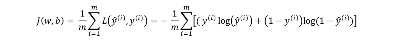
代价函数
损失函数:𝐿(𝑦̂(𝑖), 𝑦(𝑖)) = −( 𝑦(𝑖) log(𝑦̂(𝑖)) + (1 − 𝑦(𝑖))log(1 − 𝑦̂(𝑖))
代价函数:
识别猫案例
1 | import h5py |
2 | import numpy as np |
3 | |
4 | |
5 | # 加载数据 |
6 | def load_dataset(): |
7 | train_dataset = h5py.File('datasets/train_catvnoncat.h5', "r") |
8 | train_set_x_orig = np.array(train_dataset["train_set_x"][:]) # train set features |
9 | train_set_y_orig = np.array(train_dataset["train_set_y"][:]) # train set labels |
10 | test_dataset = h5py.File('datasets/test_catvnoncat.h5', "r") |
11 | test_set_x_orig = np.array(test_dataset["test_set_x"][:]) # test set features |
12 | test_set_y_orig = np.array(test_dataset["test_set_y"][:]) # test set labels |
13 | classes = np.array(test_dataset["list_classes"][:]) # the list of classes |
14 | train_set_y_orig = train_set_y_orig.reshape((1, train_set_y_orig.shape[0])) |
15 | test_set_y_orig = test_set_y_orig.reshape((1, test_set_y_orig.shape[0])) |
16 | return train_set_x_orig, train_set_y_orig, test_set_x_orig, test_set_y_orig, classes |
17 | |
18 | |
19 | # S函数 |
20 | def sigmoid(z): |
21 | return 1. / (1.+np.exp(-z)) |
22 | |
23 | |
24 | # 逻辑回归模型 |
25 | class LogisticRegression(): |
26 | def __init__(self): |
27 | pass |
28 | |
29 | # 参数初始化 |
30 | def __parameters_initializer(self, input_size): |
31 | w = np.zeros((input_size, 1), dtype=float) |
32 | b = 0.0 |
33 | return w, b |
34 | |
35 | # 前向传播 |
36 | def __forward_propagation(self, X): |
37 | A = sigmoid(np.dot(self.w.T, X) + self.b) |
38 | return A |
39 | |
40 | # 计算损失 |
41 | def __compute_cost(self, A, Y): |
42 | m = A.shape[1] |
43 | cost = -np.sum(Y*np.log(A) + (1-Y)*(np.log(1-A))) / m |
44 | return cost |
45 | |
46 | # 代价函数 |
47 | def cost_function(self, X, Y): |
48 | A = self.__forward_propagation(X) |
49 | cost = self.__compute_cost(A, Y) |
50 | return cost |
51 | |
52 | # 反向传播计算梯度 |
53 | def __backward_propagation(self, A, X, Y): |
54 | m = X.shape[1] |
55 | dw = np.dot(X, (A-Y).T) / m |
56 | db = np.sum(A-Y) / m |
57 | grads = {"dw": dw, "db": db} |
58 | return grads |
59 | |
60 | # 更新参数 |
61 | def __update_parameters(self, grads, learning_rate): |
62 | self.w -= learning_rate * grads['dw'] |
63 | self.b -= learning_rate * grads['db'] |
64 | |
65 | # 拟合 |
66 | def fit(self, X, Y, num_iterations, learning_rate, print_cost=False, print_num=100): |
67 | self.w, self.b = self.__parameters_initializer(X.shape[0]) |
68 | for i in range(num_iterations): |
69 | A = self.__forward_propagation(X) # 前行传播 |
70 | cost = self.__compute_cost(A, Y) # 计算代价 |
71 | grads = self.__backward_propagation(A, X, Y) # 后向传播计算梯度 |
72 | self.__update_parameters(grads, learning_rate) # 更新参数 |
73 | if i % print_num == 0 and print_cost: |
74 | print("Cost after iteration {}: {:.6f}".format(i, cost)) |
75 | return self |
76 | |
77 | # 预测结果的概率 |
78 | def predict_prob(self, X): |
79 | A = self.__forward_propagation(X) |
80 | return A |
81 | |
82 | # 预测结果(0 or 1) |
83 | def predict(self, X, threshold=0.5): |
84 | pred_prob = self.predict_prob(X) |
85 | threshold_func = np.vectorize(lambda x: 1 if x > threshold else 0) |
86 | Y_prediction = threshold_func(pred_prob) |
87 | return Y_prediction |
88 | |
89 | # 精度 |
90 | def accuracy_score(self, X, Y): |
91 | pred = self.predict(X) |
92 | return len(Y[pred == Y]) / Y.shape[1] |
93 | |
94 | |
95 | # 加载数据 (cat/non-cat) |
96 | train_set_x_orig, train_set_y, test_set_x_orig, test_set_y, classes = load_dataset() |
97 | m_train = train_set_x_orig.shape[0] |
98 | m_test = test_set_x_orig.shape[0] |
99 | num_px = train_set_x_orig.shape[1] |
100 | print("Number of training examples: m_train = " + str(m_train)) |
101 | print("Number of testing examples: m_test = " + str(m_test)) |
102 | print("Height/Width of each image: num_px = " + str(num_px)) |
103 | print("Each image is of size: (" + str(num_px) + ", " + str(num_px) + ", 3)") |
104 | print("train_set_x shape: " + str(train_set_x_orig.shape)) |
105 | print("train_set_y shape: " + str(train_set_y.shape)) |
106 | print("test_set_x shape: " + str(test_set_x_orig.shape)) |
107 | print("test_set_y shape: " + str(test_set_y.shape)) |
108 | |
109 | # 调整训练集与测试集数据 |
110 | train_set_x_flatten = train_set_x_orig.reshape(train_set_x_orig.shape[0], -1).T |
111 | test_set_x_flatten = test_set_x_orig.reshape(test_set_x_orig.shape[0], -1).T |
112 | print("train_set_x_flatten shape: " + str(train_set_x_flatten.shape)) |
113 | print("train_set_y shape: " + str(train_set_y.shape)) |
114 | print("test_set_x_flatten shape: " + str(test_set_x_flatten.shape)) |
115 | print("test_set_y shape: " + str(test_set_y.shape)) |
116 | print("sanity check after reshaping: " + str(train_set_x_flatten[0:5,0])) |
117 | X_train = train_set_x_flatten/255 |
118 | y_train = train_set_y |
119 | X_test = test_set_x_flatten/255 |
120 | y_test = test_set_y |
121 | |
122 | # 开始训练 |
123 | num_iter = 2001 # 迭代次数 |
124 | learning_rate = 0.005 # 学习率 |
125 | clf = LogisticRegression().fit(X_train, y_train, num_iter, learning_rate, True, 500) |
126 | train_acc = clf.accuracy_score(X_train, y_train) |
127 | print('training acc: {}'.format(train_acc)) |
128 | test_acc = clf.accuracy_score(X_test, y_test) |
129 | print('testing acc: {}'.format(test_acc)) |
- 输出结果
1 | Cost after iteration 0: 0.693147 |
2 | Cost after iteration 500: 0.303273 |
3 | Cost after iteration 1000: 0.214820 |
4 | Cost after iteration 1500: 0.166521 |
5 | Cost after iteration 2000: 0.135608 |
6 | training acc: 0.9904306220095693 |
7 | testing acc: 0.7 |
